Application: Training Physics-Informed Neural Networks (PINNs).

In this example, we will train a neural network to solve a partial differential equation (PDE). The PDE's Physics are incorporated into the loss function via derivatives that we will compute with Taylor mode. This is known as a Physics-Informed Neural Networks (PINNs).

Let's get the imports out of the way.

from math import log10, pi, sqrt
from shutil import which
from time import time

from hessianfree.optimizer import HessianFree
from matplotlib import pyplot as plt
from torch import (
    Tensor,
    cat,
    float64,
    manual_seed,
    no_grad,
    prod,
    rand,
    randint,
    sin,
    vmap,
    zeros,
)
from torch.nn import Linear, Sequential, Tanh
from torch.optim import Adam
from tueplots import bundles

from jet.laplacian import laplacian
from jet.simplify import common_subexpression_elimination
from jet.tracing import capture_graph

_ = manual_seed(42)  # make deterministic

DTYPE = float64  # we want to learn an accurate solution, hence we use double precision

2d Poisson equation

Setup

We will consider the Poisson equation on the two-dimensional unit square $\Omega = [0; 1]^2$ with zero boundary conditions on $\partial \Omega$. from Mueller, Zeinhofer, ICML 2023 as a simple example. $$ \text{Interior:} \quad - \Delta f(x, y) = 2 \pi^2 \sin (\pi x) \sin (\pi y) \quad (x, y) \in \Omega = [0; 1]^2\,, $$ $$ \text{Boundary:} \quad f(x, y) = 0 \quad (x, y) \in \partial \Omega = \partial [0;1]^2\,. $$ The known solution, later used for verification, is: $$ f^\star(x, y) = \sin(\pi x) \sin(\pi y)\,. $$

@vmap
def f_star(x: Tensor) -> Tensor:
    """Evaluate the exact solution to the Poisson equation.

    Args:
        x: A tensor with two entries, the (x, y) coordinates.

    Returns:
        The exact solution to the Poisson equation evaluated at (x, y). Has shape `[1]`.
    """
    assert x.shape == (2,)
    return prod(sin(pi * x), 0, keepdim=True)

To approximate $f^\star$, we use a neural network $f_\mathbf{\theta}$ with parameters $\mathbf{\theta}$, in our case a $2 \to 64 \to 1$ MLP with tanh activation:

f = Sequential(Linear(2, 64), Tanh(), Linear(64, 1)).to(DTYPE)

To assess the accuracy of the neural network's learned solution, we compute the root mean square error (also known as L$_2$ error) on a test set of 9,000 points.

N_test = 9_000
X_test = rand(N_test, 2, dtype=DTYPE)


@no_grad()
def l2_error() -> Tensor:
    """Compute the root mean square error ('test error').

    Returns:
        The root mean square error. Has shape `[1]`.
    """
    return ((f(X_test) - f_star(X_test)) ** 2).mean(0).sqrt()


print(f"Initial L2 error: {l2_error().item():.2e}")

Out:

Initial L2 error: 3.96e-01

To train the neural network, we use a loss that enforces both the interior and the boundary conditions to hold. The total loss consists of two parts, the interior and the boundary loss $$ \mathcal{L}(\mathbf{\theta}) = \mathcal{L}_{\Omega}(\mathbf{\theta}) + \mathcal{L}_{\partial \Omega}(\mathbf{\theta})\,, $$ with interior loss ($(x_i, y_i) \sim \Omega$) $$ \mathcal{L}_\Omega(\mathbf{\theta}) = \frac{1}{2 N_{\Omega}} \sum_{i=1}^{N_{\Omega}} \left\lVert \Delta f_{\mathbf{\theta}}(x_i, y_i) + 2 \pi^2 \sin(\pi x_i) \sin(\pi y_i) \right\rVert^2\,, $$ and boundary loss ($(x_j^\partial, y_j^\partial) \sim \partial \Omega$) $$ \mathcal{L}_{\partial\Omega}(\mathbf{\theta}) = \frac{1}{2 N_{\partial\Omega}} \sum_{i=1}^{N_{\partial \Omega}} \left\lVert f_{\mathbf{\theta}}(x_j^\partial, y_j^\partial) \right\rVert^2\,. $$ We can combine both losses into a single square loss, $\mathcal{L}(\mathbf{\theta}) = \frac{1}{2} \lVert \mathbf{r} \rVert^2$, with the residual $$ \mathbf{r} = \begin{pmatrix} \frac{1}{\sqrt{N_{\partial\Omega}}} f_{\mathbf{\theta}}(x_1^\partial, y_1^\partial) \\ \vdots \\ \frac{1}{\sqrt{N_{\partial\Omega}}} f_{\mathbf{\theta}}(x_{N_{\partial \Omega}}^\partial, y_{N_{\partial \Omega}}^\partial) \\ \frac{1}{\sqrt{N_\Omega}} \left( \Delta f_{\mathbf{\theta}}(x_1, y_1) + 2 \pi^2 \sin(\pi x_1) \sin(\pi y_1) \right) \\ \vdots \\ \frac{1}{\sqrt{N_\Omega}} \left( \Delta f_{\mathbf{\theta}}(x_{N_{\Omega}}, y_{N_{\Omega}}) + 2 \pi^2 \sin(\pi x_{N_{\Omega}}) \sin(\pi y_{N_{\Omega}}) \right) \end{pmatrix} $$ so we can think about this problem as a standard regression task.

Let's draw the data points that we will train on, then write a function that computes the loss

# Draw points from the domain
N_interior = 900
X_interior = rand(N_interior, 2, dtype=DTYPE)


# Draw points from the domain's boundary
N_boundary = 120


def sample_boundary(N: int = N_boundary) -> Tensor:
    """Uniformly sample points from the boundary of the unit square [0,1]^2.

    Args:
        N: Number of points to sample. Default: `120`.

    Returns:
        Tensor of shape `[N, 2]` containing points on the boundary.
    """
    # 4 edges, each with equal probability
    edges = randint(0, 4, (N,))

    # Uniform coordinate values
    coords = rand(N, dtype=DTYPE)

    # Initialize tensor
    points = zeros(N, 2, dtype=DTYPE)

    # Assign coordinates based on which edge is chosen
    # 0: bottom (y=0), 1: top (y=1), 2: left (x=0), 3: right (x=1)
    bottom = edges == 0
    top = edges == 1
    left = edges == 2
    right = edges == 3

    points[bottom, 0] = coords[bottom]
    points[bottom, 1] = 0

    points[top, 0] = coords[top]
    points[top, 1] = 1

    points[left, 0] = 0
    points[left, 1] = coords[left]

    points[right, 0] = 1
    points[right, 1] = coords[right]

    return points


X_boundary = sample_boundary()

With that, we can write functions that compute the loss. Note that we need to compute the neural network's Laplacian for the interior loss, as well as the Poisson equation's right-hand side.

# Function that computes the neural network's Laplacian
lap_f = laplacian(f, (zeros(2, dtype=DTYPE),))  # uses collapsed Taylor mode
# Capture the operator's graph so we can apply CSE + dead code elimination.
lap_f, _ = capture_graph(lap_f, (zeros(2, dtype=DTYPE),))
common_subexpression_elimination(lap_f.graph)
lap_f.recompile()
lap_f = vmap(lap_f)  # parallelized over data points


@vmap
def rhs(x: Tensor) -> Tensor:
    """Evaluate the right hand side of the Poisson equation.

    Args:
        x: A tensor with two entries, the (x, y) coordinates.

    Returns:
        The Poisson equation's right hand side. Has shape `[1]`,
    """
    assert x.shape == (2,)
    return 2 * pi**2 * prod(sin(pi * x), 0, keepdim=True)


rhs_interior = rhs(X_interior)


def compute_loss(return_residual: bool = False) -> Tensor | tuple[Tensor, Tensor]:
    """Compute the Physics-informed loss.

    Args:
        return_residual: Whether to return the residual along with the loss.
            Defaults to `False`.

    Returns:
        The loss. If `return_residual` is `True`, returns a tuple of the loss and the
        residual. The loss has shape `[1]`, the residual `[N_interior + N_boundary]`.
    """
    boundary_residual = f(X_boundary) / sqrt(N_boundary)
    interior_residual = (lap_f(X_interior) + rhs(X_interior)) / sqrt(N_interior)
    residual = cat([interior_residual, boundary_residual])
    loss = 0.5 * (residual**2).sum()
    return (loss, residual) if return_residual else loss


print(f"Initial loss: {compute_loss().item():.2e}")

Out:

Initial loss: 4.54e+01

Training utilities

We need some helper functions to orchestrate training and logging. Feel free to skip them.

original_params = [p.clone() for p in f.parameters()]


def reset_model():
    """Resets the neural network parameters to their original values."""
    for p, orig_p in zip(f.parameters(), original_params):
        p.data = orig_p.data.clone()


class Timer:
    """A class for measuring elapsed time."""

    def __init__(self):
        """Initialize the timer."""
        self._start_time = None
        self._elapsed = 0.0
        self._running = False

    def start(self):
        """Start or resume the timer."""
        if not self._running:
            self._start_time = time()
            self._running = True

    def pause(self):
        """Pause the timer (accumulate elapsed time)."""
        if self._running:
            self._elapsed += time() - self._start_time
            self._running = False

    def elapsed(self) -> float:
        """Return total elapsed time in seconds.

        Returns:
            Elapsed time in seconds.
        """
        return (
            self._elapsed + (time() - self._start_time)
            if self._running
            else self._elapsed
        )


def milestone(n: int) -> bool:
    """Check if n is a logging milestone.

    Args:
        n: The current step.

    Returns:
        Whether n is a logging milestone.
    """
    assert n > 0 and isinstance(n, int)
    step = 10 ** int(log10(n))
    return n % step == 0

Training

We will compare training the PINN with different algorithms. Each algorithm is allowed a compute time budget (excluding the validation time).

T_MAX = 10  # training budget in seconds

With Adam

Let's start with Adam.

adam = Adam(f.parameters())

# logged quantities
adam_time, adam_step, adam_l2 = [], [], []

print(f"Training with {adam.__class__.__name__}")
timer = Timer()
steps = 0
timer.start()

while timer.elapsed() < T_MAX:
    # training step
    adam.zero_grad()
    loss = compute_loss()
    loss.backward()
    adam.step()
    steps += 1

    # logging
    if milestone(steps) or timer.elapsed() >= T_MAX:
        timer.pause()
        adam_time.append(timer.elapsed())
        adam_step.append(steps)
        l2 = l2_error().item()
        loss = loss.item()
        adam_l2.append(l2)
        print(f"\t{steps=}, {timer.elapsed():.2f}s, {loss=:.2e}, {l2=:.2e}")
        timer.start()

Out:

Training with Adam
        steps=1, 0.01s, loss=4.54e+01, l2=4.10e-01
        steps=2, 0.02s, loss=4.53e+01, l2=4.25e-01
        steps=3, 0.02s, loss=4.52e+01, l2=4.40e-01
        steps=4, 0.03s, loss=4.51e+01, l2=4.55e-01
        steps=5, 0.04s, loss=4.50e+01, l2=4.70e-01
        steps=6, 0.05s, loss=4.49e+01, l2=4.86e-01
        steps=7, 0.06s, loss=4.49e+01, l2=5.01e-01
        steps=8, 0.06s, loss=4.48e+01, l2=5.17e-01
        steps=9, 0.07s, loss=4.47e+01, l2=5.32e-01
        steps=10, 0.08s, loss=4.46e+01, l2=5.48e-01
        steps=20, 0.12s, loss=4.36e+01, l2=7.01e-01
        steps=30, 0.16s, loss=4.26e+01, l2=8.50e-01
        steps=40, 0.19s, loss=4.16e+01, l2=9.94e-01
        steps=50, 0.23s, loss=4.06e+01, l2=1.14e+00
        steps=60, 0.27s, loss=3.95e+01, l2=1.28e+00
        steps=70, 0.31s, loss=3.83e+01, l2=1.42e+00
        steps=80, 0.34s, loss=3.71e+01, l2=1.56e+00
        steps=90, 0.38s, loss=3.58e+01, l2=1.71e+00
        steps=100, 0.42s, loss=3.45e+01, l2=1.84e+00
        steps=200, 0.76s, loss=2.07e+01, l2=2.31e+00
        steps=300, 1.09s, loss=1.17e+01, l2=1.26e+00
        steps=400, 1.42s, loss=8.15e+00, l2=3.71e-01
        steps=500, 1.76s, loss=6.25e+00, l2=3.34e-01
        steps=600, 2.10s, loss=4.39e+00, l2=4.01e-01
        steps=700, 2.45s, loss=2.63e+00, l2=4.49e-01
        steps=800, 2.81s, loss=1.37e+00, l2=4.26e-01
        steps=900, 3.17s, loss=7.19e-01, l2=3.31e-01
        steps=1000, 3.53s, loss=4.30e-01, l2=2.35e-01
        steps=2000, 7.00s, loss=1.02e-01, l2=7.25e-02
        steps=2808, 10.00s, loss=4.84e-02, l2=5.75e-02

With the Hessian-free optimizer

Next, we use a second-order method, the Hessian-free optimizer from Martens, ICML 2010, based on Lukas Tatzel's PyTorch implementation. Because the loss landscape of PINNs is known to be challenging for first-order methods like Adam, second-order methods often converge faster, or yield better accuracy. The Hessian-free (HF) optimizer is based on the Gauss-Newton method and requires access to the residual.

Here is the training loop:

reset_model()
hf = HessianFree(f.parameters())

# logged quantities
hf_time, hf_step, hf_l2 = [], [], []

print(f"Training with {hf.__class__.__name__}")
timer = Timer()
steps = 0
timer.start()

while timer.elapsed() < T_MAX:
    # training step
    loss = hf.step(lambda: compute_loss(return_residual=True))
    steps += 1

    # logging
    if milestone(steps) or timer.elapsed() >= T_MAX:
        timer.pause()
        hf_time.append(timer.elapsed())
        hf_step.append(steps)
        l2 = l2_error().item()
        hf_l2.append(l2)
        print(f"\t{steps=}, {timer.elapsed():.2f}s, {loss=:.2e}, {l2=:.2e}")
        timer.start()

Out:

Training with HessianFree
        steps=1, 0.11s, loss=1.46e+01, l2=1.30e+00
        steps=2, 0.29s, loss=1.40e+01, l2=2.68e-01
        steps=3, 0.50s, loss=1.24e+01, l2=4.27e-01
        steps=4, 0.71s, loss=6.64e+00, l2=1.06e+00
        steps=5, 0.93s, loss=6.41e+00, l2=4.74e-01
        steps=6, 1.19s, loss=2.02e+00, l2=1.88e-01
        steps=7, 1.47s, loss=1.38e+00, l2=1.46e-01
        steps=8, 1.75s, loss=3.50e-01, l2=1.51e-01
        steps=9, 2.04s, loss=2.87e-01, l2=1.18e-01
        steps=10, 2.32s, loss=2.46e-01, l2=1.15e-01
/home/docs/checkouts/readthedocs.org/user_builds/torch-jet/envs/latest/lib/python3.12/site-packages/hessianfree/optimizer.py:506: UserWarning: The reduction ratio `rho` is negative. This might result in a bad cg-initialization in the next step.
  warn(msg)
        steps=20, 6.45s, loss=2.45e-02, l2=5.00e-02
        steps=27, 10.08s, loss=3.21e-04, l2=4.81e-03

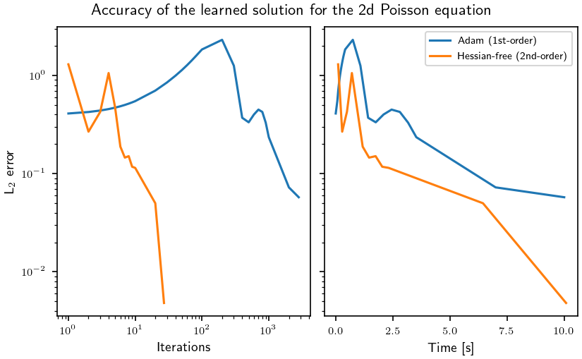
Indeed, training with the Hessian-free optimizer outperforms Adam:

# Use LaTeX if available
USETEX = which("latex") is not None

with plt.rc_context(bundles.neurips2024(usetex=USETEX)):
    fig, ax = plt.subplots(ncols=2, sharey=True, dpi=150)
    ax[0].set_ylabel("L$_2$ error")
    ax[0].set_xlabel("Iterations")
    ax[1].set_xlabel("Time [s]")
    fig.suptitle("Accuracy of the learned solution for the 2d Poisson equation")

    ax[0].loglog(adam_step, adam_l2)
    ax[1].semilogy(adam_time, adam_l2, label="Adam (1st-order)")

    ax[0].loglog(hf_step, hf_l2)
    ax[1].semilogy(hf_time, hf_l2, label="Hessian-free (2nd-order)")

    ax[1].legend()

assert adam_l2[-1] > hf_l2[-1]