Note
Click here to download the full example code
Introduction to Taylor Mode.
This example provides an introduction to Taylor Mode, specifically the jet function
transformation, and how to use it to compute higher-order derivatives.
We will focus on second-order derivatives.
First, the imports.
from os import path

from pytest import raises
from torch import Tensor, cos, manual_seed, ones_like, rand, sin, zeros_like
from torch.func import hessian
from torch.nn import Linear, Sequential, Tanh

from jet import capture_graph, jet, visualize_graph

# Use the Taylor-mode concept diagram (shown below) as the gallery thumbnail.
# Path is relative to the mkdocs ``docs_dir``.
# mkdocs_gallery_thumbnail_path = 'examples/01_taylor_mode.png'

HEREDIR = path.dirname(path.abspath(__name__))
# We need to store figures here so they will be picked up in the built doc
GALLERYDIR = path.join(path.dirname(HEREDIR), "generated", "gallery")

_ = manual_seed(0)  # make deterministic
What Is Taylor Mode?
Taylor mode is an autodiff technique for efficiently computing higher-order derivatives of functions. The basic idea is described by the following diagram (taken from the paper):
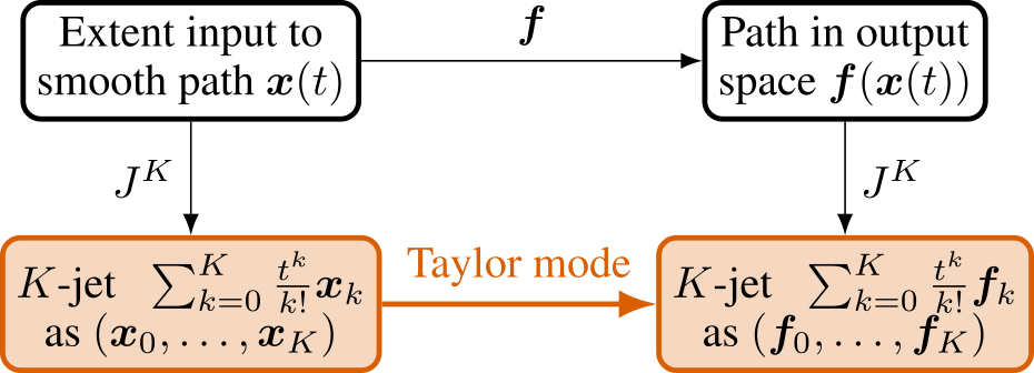
Let's walk through this diagram for the example of a scalar function \(f : \mathbb{R} \to \mathbb{R}, x \mapsto f(x)\) and assume we want to evaluate the function or its derivatives at a point \(x_0 \in \mathbb{R}\).
-
Top left: Instead of considering a point \(x_0\) in input space, let us instead consider a curve \(x(t)\), where \(t \in \mathbb{R}\) is time. Importantly, this curve has to intersect the anchor when \(t=0\), or \(x(0) = x_0\).
-
Top left \(\to\) right: Clearly, the curve \(x(t)\) in the input space gives rise to a curve \(f(x(t))\) in the output space. Our goal is to extract information about the output curve given information about the input curve.
-
Left top \(\to\) bottom: So, how do derivatives come into play? The answer is that derivatives naturally allow us to control properties of the curve \(x(t)\). Let's say we want to control the curve's velocity, acceleration, etc. at the anchor point. We can do this by writing out the curve's Taylor expansion $$ x(t) = x_0 + x_1 t + \frac{1}{2} x_2 t^2 + \ldots $$ where \(x_0\) is the anchor point, \(x_1\) is the velocity at the anchor, \(x_2\) is the acceleration, and so on. We call \((x_0, x_1, x_2)\) the 2-jet of \(x(t)\), and \(x_i = \left.\frac{\mathrm{d}^i x(t)}{\mathrm{d} t^i}\right|_{t=0}\) the \(i\)th Taylor coefficient.
-
Right top \(\to\) bottom: Just like for the input curve, we can also write the Taylor expansion of the output curve \(f(x(t))\) at the anchor point: $$ f(x(t)) = f_0 + f_1 t + \frac{1}{2} f_2 t^2 + \ldots $$ where \((f_0, f_1, f_2)\) is the 2-jet of \(f(x(t))\) and the \(i\)th Taylor coefficient is \(f_i = \left.\frac{\mathrm{d}^i f(x(t))}{\mathrm{d} t^i}\right|_{t=0}\).
-
Bottom left \(\to\) right: The question is now how we can compute the 2-jet of the output curve \(f(x(t))\) given the 2-jet of the input curve \(x(t)\). This is exactly what Taylor mode does!
The propagation rules are relatively easy to derive by hand using the chain rule:
$$ \begin{matrix} f_0 =& \left.\frac{\mathrm{d}^0 f(x(t))}{\mathrm{d} t^0}\right|_{t=0} =& f(x_0) \\ f_1 =& \left.\frac{\mathrm{d} f(x(t))}{\mathrm{d} t}\right|_{t=0} =& f'(x_0) x_1 \\ f_2 =& \left.\frac{\mathrm{d}^2 f(x(t))}{\mathrm{d} t^2}\right|_{t=0} =& f''(x_0) x_2 + f'(x_0) x_1^2 \\ \vdots \end{matrix} $$ See the paper's appendix for a cheat sheet that contains even higher orders. The important insight is that, by specifying the Taylor coefficients \((x_0, x_1, \dots)\), we can compute various derivatives!
In code, the jet library offers a function transformation
jet(f, mock_args) that takes a function \(f\) and mock primal inputs and
returns a new function jet_f(*args) taking one argument per argument of
\(f\). Each argument bundles a primal with its Taylor coefficients into a
tuple (x_0, x_1, ..., x_K), and the output mirrors this: each result is a
tuple (f_0, f_1, ..., f_K) holding the function value and its Taylor
coefficients up to that derivative order. The order \(K\) is inferred per
call from the input — the returned jet_f works at any \(K\).
Scalar-to-scalar Function
Let's make computing higher-order derivatives with Taylor mode concrete, sticking to the scalar case from a above with a function \(f : \mathbb{R} \to \mathbb{R}\). We will illustrate how to compute the second-order derivative \(f''(x)\), and hence use the 2-jet of \(f\), whose propagation is (re-stated from above) $$ f_{2\text{-jet}}: \begin{pmatrix} x_0 \\ x_1 \\ x_2 \end{pmatrix} \mapsto \begin{pmatrix} f_0 = & f(x_0) \\ f_1 = & f'(x_0) x_1 \\ f_2 = & f''(x_0) x_1^2 + f'(x_0) x_2 \end{pmatrix}\,. $$ To achieve our goal, note that we can compute the second-order derivative \(f''(x)\), by setting \(x_0 = x\), \(x_1 = 1\), and \(x_2 = 0\), which yields \(f_2 = f''(x)\):
# Define a function and obtain its jet function
f = sin  # propagates x₀ ↦ f(x₀)
x = rand(1)
f_jet = jet(f, (x,))  # propagates (x₀, x₁, ..., x_K) ↦ (f₀, f₁, ..., f_K)

# Set up the Taylor coefficients to compute the second derivative

x0 = x
x1 = ones_like(x)
x2 = zeros_like(x)

# Evaluate the second derivative
f0, f1, f2 = f_jet((x0, x1, x2))
Let's verify that this indeed yields the correct result:
# Compare to the second derivative computed with first-order autodiff
d2f = hessian(f)(x)

if f2.allclose(d2f):
    print("Taylor mode Hessian matches functorch Hessian!")
else:
    raise ValueError(f"{f2} does not match {d2f}!")

# We know the sine function's second derivative, so let's also compare with that
d2f_manual = -sin(x)
if f2.allclose(d2f_manual):
    print("Taylor mode Hessian matches manual Hessian!")
else:
    raise ValueError(f"{f2} does not match {d2f_manual}!")
Out:
/home/docs/checkouts/readthedocs.org/user_builds/torch-jet/envs/latest/lib/python3.12/site-packages/torch/jit/_script.py:1488: DeprecationWarning: `torch.jit.script` is deprecated. Please switch to `torch.compile` or `torch.export`.
  warnings.warn(
Taylor mode Hessian matches functorch Hessian!
Taylor mode Hessian matches manual Hessian!
Vector-to-scalar Function
Next, let's consider a vector to-scalar-function \(f : \mathbb{R}^D \to \mathbb{R}\), \(\mathbf{x} \mapsto f(\mathbf{x})\) (for the most general, please see the paper). We can do the exact derivation as above to obtain the output jets $$ f_{2\text{-jet}}: \begin{pmatrix} \mathbf{x}_0 \\ \mathbf{x}_1 \\ \mathbf{x}_2 \end{pmatrix} \mapsto \begin{pmatrix} f_0 = & f(\mathbf{x}_0) \\ f_1 = & (\nabla f(\mathbf{x}_0))^\top \mathbf{x}_1 \\ f_2 = & \mathbf{x}_1^\top (\nabla^2 f(\mathbf{x}_0)) \mathbf{x}_1 + (\nabla f(\mathbf{x}_0))^\top \mathbf{x}_2 \end{pmatrix}\,, $$ where \(\nabla f(\mathbf{x}_0) \in \mathbb{R}^D\) is the gradient, and \(\nabla^2 f(\mathbf{x}_0) \in \mathbb{R}^{D\times D}\) the Hessian, of \(f\) at \(\mathbf{x}_0\), while \(\mathbf{x}_i\) is the \(i\)th input space Taylor coefficient. If we set \(\mathbf{x}_0 = \mathbf{x}\), \(\mathbf{x}_2 = \mathbf{0}\), then we can compute vector-Hessian-vector products (VHVPs) of the form $$ f_2 = \mathbf{v}^\top (\nabla^2 f(\mathbf{x})) \mathbf{v} $$ by setting \(\mathbf{x}_1 = \mathbf{v}\). One interesting example is setting \(\mathbf{x}_1 = \mathbf{e}_i\) to the \(i\)th canonical basis vector, which yields the \(i\)th diagonal entry of the Hessian, i.e., $$ [\nabla^2 f(\mathbf{x})]_{i,i} = \mathbf{e}_i^\top (\nabla^2 f(\mathbf{x})) \mathbf{e}_i\,. $$
Let's try this out and compute the Hessian diagonal with Taylor mode. This time, we will use a neural network with \(\mathrm{tanh}\) activations:
D = 3
f = Sequential(Linear(D, 1), Tanh())
x = rand(D)
f_jet = jet(f, (x,))

# constant Taylor coefficients
x0 = x
x2 = zeros_like(x)

d2_diag = zeros_like(x)

# Compute the d-th diagonal element of the Hessian
for d in range(D):
    x1 = zeros_like(x)
    x1[d] = 1.0  # d-th canonical basis vector
    f0, f1, f2 = f_jet((x0, x1, x2))
    d2_diag[d] = f2
Let's compare this to computing the Hessian with functorch and then taking its
diagonal:
d2f = hessian(f)(x)  # has shape [1, D, D]
hessian_diag = d2f.squeeze(0).diag()

if d2_diag.allclose(hessian_diag):
    print("Taylor mode Hessian diagonal matches functorch Hessian diagonal!")
else:
    raise ValueError(f"{d2_diag} does not match {hessian_diag}!")
Out:
Multi-variate Functions
So far, we have applied jet to functions with a single tensor argument. But jet
also supports functions with multiple inputs. This is useful, for example, when
dealing with partial differential equations (PDEs) where the unknown depends on
multiple variables such as time and space.
For a function with multiple arguments, mock_args is a tuple that matches the
function's positional arguments, and the jet is called as jet_f(*args) with one
argument per argument of \(f\). Each argument bundles its primal with its Taylor
coefficients as a tuple (x_0, x_1, ..., x_K).
.. note::
**Comparison with JAX's Taylor mode.**
`JAX's jet <https://docs.jax.dev/en/latest/jax.experimental.jet.html>`_
uses the signature ``jet(fun, primals, series)`` where ``primals`` and
``series`` are kept as *separate* arguments. ``torch-jet`` instead bundles
each primal with its Taylor coefficients into a single ``(x_0, x_1, ...)``
tuple per argument, so a jet is one self-contained object.

A further difference is that ``torch-jet`` uses a two-step API: first
``jet_f = jet(f, mock_args)`` traces the function, then ``jet_f(*args)``
evaluates it. This separates tracing (which can be expensive) from
evaluation, allowing the traced jet to be reused across multiple inputs
and across any derivative order $K$ (inferred per call from the input).
As a concrete example, consider the function
\(u(t, x) = \cos(t) \sin(x)\), which is a solution to the 1-D wave equation
\(\partial_{tt} u = \partial_{xx} u\). We will use jet to compute
\(\partial_{tt} u\) and \(\partial_{xx} u\) and verify the wave equation.
def u(t: Tensor, x: Tensor) -> Tensor:
    """A solution to the 1-D wave equation.

    Args:
        t: Time (scalar tensor).
        x: Space (scalar tensor).

    Returns:
        u(t, x) = cos(t) * sin(x).
    """
    return cos(t) * sin(x)


t0, x0 = rand(1), rand(1)  # evaluation point
u_jet = jet(u, (t0, x0))
Computing \(\partial_{xx} u\). We set \(t_1 = 0\), \(x_1 = 1\), \(t_2 = 0\), \(x_2 = 0\) so that \(f_2 = \partial_{xx} u\):
t1, t2 = zeros_like(t0), zeros_like(t0)  # t_1 = 0, t_2 = 0
x1, x2 = ones_like(x0), zeros_like(x0)  # x_1 = 1, x_2 = 0
_, _, d2u_dx2 = u_jet((t0, t1, t2), (x0, x1, x2))

d2u_dx2_exact = -cos(t0) * sin(x0)
if d2u_dx2.allclose(d2u_dx2_exact):
    print("∂²u/∂x² matches analytical value!")
else:
    raise ValueError(f"∂²u/∂x² = {d2u_dx2} does not match {d2u_dx2_exact}")
Out:
Similarly, \(\partial_{tt} u\) is obtained with \(t_1 = 1\), \(x_1 = 0\). Let's verify the wave equation \(\partial_{tt} u = \partial_{xx} u\):
t1, t2 = ones_like(t0), zeros_like(t0)  # t_1 = 1, t_2 = 0
x1, x2 = zeros_like(x0), zeros_like(x0)  # x_1 = 0, x_2 = 0
_, _, d2u_dt2 = u_jet((t0, t1, t2), (x0, x1, x2))

if d2u_dt2.allclose(d2u_dx2):
    print("Wave equation verified: ∂²u/∂t² = ∂²u/∂x²!")
else:
    raise ValueError(f"∂²u/∂t² = {d2u_dt2} does not match ∂²u/∂x² = {d2u_dx2}")
Out:
Pytree Inputs and Outputs
jet also supports functions whose inputs and outputs are arbitrary pytrees
(nested tuple, list, and dict containers with tensor leaves). As an
example, consider a function that takes a dict with entries "x" and "y"
and returns a dict with entries "mul" and "sub":
def f_pytree(inputs: dict[str, Tensor]) -> dict[str, Tensor]:
    """A function with dict input and dict output.

    Args:
        inputs: A dict with keys ``"x"`` and ``"y"``, each a tensor.

    Returns:
        A dict with ``"mul" = x * y`` and ``"sub" = x - y``.
    """
    x, y = inputs["x"], inputs["y"]
    return {"mul": x * y, "sub": x - y}


mock_inputs = {"x": rand(2), "y": rand(2)}
f_pytree_jet = jet(f_pytree, (mock_inputs,))
The jet of a pytree argument follows the same pytree structure as the argument
itself, with every tensor leaf replaced by its (primal, c_1, ..., c_K) jet
tuple. Since f_pytree takes a single dict argument, we pass a single dict
whose "x" and "y" leaves are each a (primal, c_1) tuple (one Taylor
coefficient — the order K is inferred from the input):
inputs = {"x": rand(2), "y": rand(2)}
d_inputs = {"x": ones_like(inputs["x"]), "y": zeros_like(inputs["y"])}

jet_inputs = {
    "x": (inputs["x"], d_inputs["x"]),
    "y": (inputs["y"], d_inputs["y"]),
}
out = f_pytree_jet(jet_inputs)
The output mirrors f_pytree's output structure (a dict), with each leaf a
(f_0, f_1) jet tuple:
print(f"output keys: {list(out.keys())}")
print(f"out['mul'][1] = {out['mul'][1]}  (= dx/dt * y + x * dy/dt = 1 * y + x * 0 = y)")
print(f"out['sub'][1] = {out['sub'][1]}  (= dx/dt - dy/dt = 1 - 0 = 1)")

assert out["mul"][1].allclose(inputs["y"]), f"out['mul'][1] = {out['mul'][1]} != y"
assert out["sub"][1].allclose(ones_like(inputs["x"])), "out['sub'][1] != 1"
Out:
output keys: ['mul', 'sub']
out['mul'][1] = tensor([0.6977, 0.8000])  (= dx/dt * y + x * dy/dt = 1 * y + x * 0 = y)
out['sub'][1] = tensor([1., 1.])  (= dx/dt - dy/dt = 1 - 0 = 1)
Supported Operations
Taylor mode works by overloading the ATen operators that PyTorch lowers a
function to. The set of operators we have a jet rule for lives in the registry
jet._rules.RULES (a dict keyed by ATen op overloads). Any function that
traces down to these operators is supported. The list below is generated
live from the registry, so it always reflects the current coverage:
from jet._rules import RULES  # noqa: E402

print("Supported ATen operators:")
for op in sorted(str(key) for key in RULES):
    print(f"  - {op}")
Out:
Supported ATen operators:
  - aten._adaptive_avg_pool2d.default
  - aten._log_softmax.default
  - aten._unsafe_view.default
  - aten.add.Tensor
  - aten.addmm.default
  - aten.avg_pool2d.default
  - aten.cat.default
  - aten.convolution.default
  - aten.cos.default
  - aten.div.Scalar
  - aten.div.Tensor
  - aten.exp.default
  - aten.log.default
  - aten.max_pool2d.default
  - aten.max_pool2d_with_indices.default
  - aten.mean.default
  - aten.mean.dim
  - aten.mm.default
  - aten.mse_loss.default
  - aten.mul.Tensor
  - aten.native_batch_norm.default
  - aten.neg.default
  - aten.nll_loss_forward.default
  - aten.pow.Tensor_Scalar
  - aten.relu.default
  - aten.sigmoid.default
  - aten.sin.default
  - aten.squeeze.dim
  - aten.squeeze.dims
  - aten.stack.default
  - aten.sub.Tensor
  - aten.sum.default
  - aten.sum.dim_IntList
  - aten.t.default
  - aten.tanh.default
  - aten.unsqueeze.default
  - aten.view.default
  - aten.zeros_like.default
Conclusion
If your goal was to learn how to use the jet function, you can stop reading at this point.
But if you are interested in how jet works under the hood, and what its limitations
are, keep reading!
How It Works
jet uses make_fx to capture the function's ATen-level compute graph, then
runs it through a JetInterpreter that dispatches jet operations (e.g.
jet_linear, jet_tanh) in place of the original ATen ops. jet itself
returns a plain Python callable; we can optionally capture its graph with
capture_graph to obtain a torch.fx.GraphModule containing the fully
unrolled jet computation, suitable for graph-level passes like common
subexpression elimination.
Let's visualize both the original function's compute graph and the jet function:
mod, in_spec = capture_graph(f, (x,))
visualize_graph(mod, path.join(GALLERYDIR, "01_f.png"))
f_val = mod(*in_spec.flatten_up_to((x,)))
assert f_val.allclose(f(x))

# Capture the jet's graph at K=2 by passing a representative mock 2-jet tuple.
mock_2jet = (x, zeros_like(x), zeros_like(x))
f_2jet_mod, in_spec = capture_graph(f_jet, (mock_2jet,))
visualize_graph(f_2jet_mod, path.join(GALLERYDIR, "01_f_jet.png"))
x_2jet = (x, ones_like(x), zeros_like(x))
f_2jet_val = f_2jet_mod(*in_spec.flatten_up_to((x_2jet,)))
assert f_2jet_val[2].allclose(f_jet(x_2jet)[2])
The returned GraphModule's forward takes the flat tensor leaves
of mock_args (not the original pytree). Use the second return value,
in_spec, to flatten new arguments in the order the graph expects.
| Original function \(f\) | 2-jet function \(f_{2\text{-jet}}\) |
|---|---|
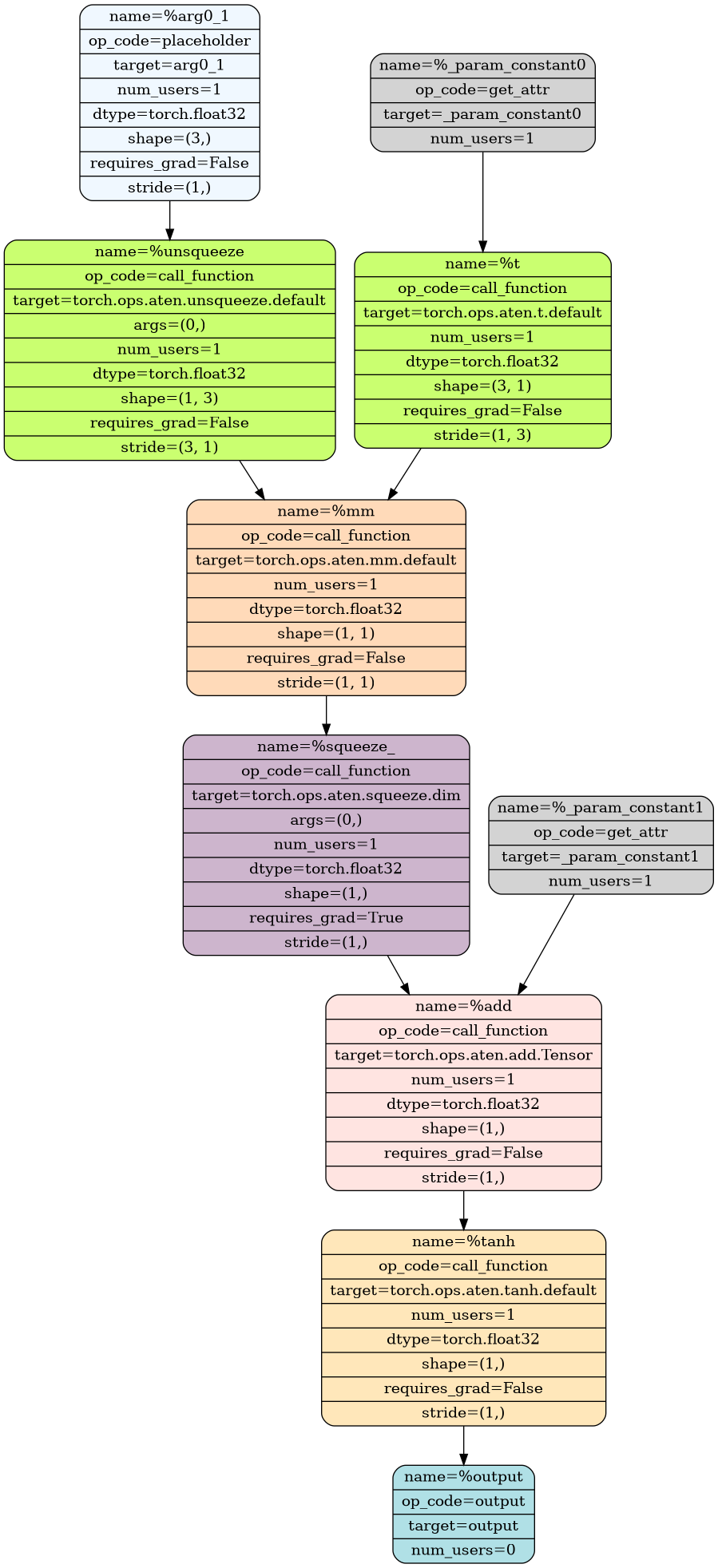 |
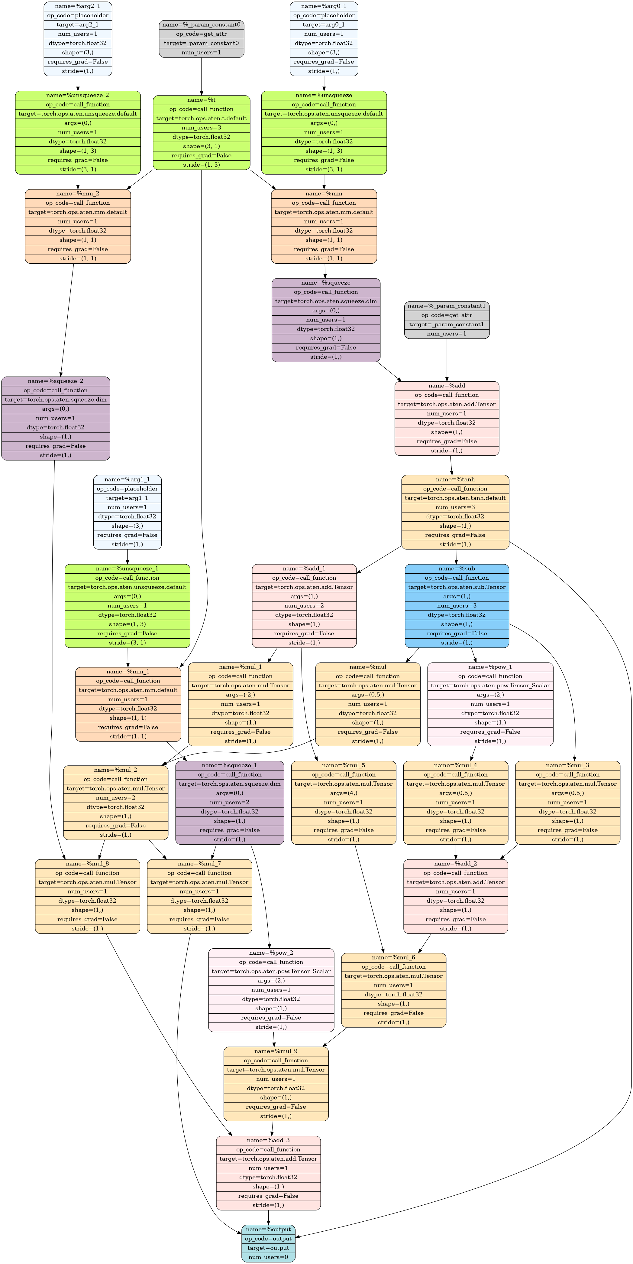 |
The unrolled graph is, unsurprisingly, much larger. However, you should be able to
recognize all functions that are being called. We can regard this process as a
cycle that starts with a function \(f\) that uses operations from PyTorch, and ends
with a function \(f_{k\text{-jet}}\) that also uses PyTorch operations.
This is a desirable property as it enables composability (e.g. taking the jet of
a jet).
Limitations
Our jet implementation for PyTorch that this library provides has various
limitations. Here, we want to describe them and comment on the potential to fix them.
Some limitations are a consequence of our still evolving know-how
how to properly implement jet in PyTorch. So if you have suggestions how to fix
them, please reach out to us, open an issue, or submit a pull request  .
.
Untraceable Functions
jet inherits all limitations of make_fx tracing.
We need to capture the function's compute graph to overload it to obtain a jet.
We use make_fx to achieve this. It has certain limitations
(please see the documentation) that our jet implementation inherits.
For instance, data-dependent control flow cannot be traced:
def f(x: Tensor):
    """Function with data-dependent control flow (if statement).

    Args:
        x: Input tensor.

    Returns:
        The sine of x if the sum of x is positive, otherwise the cosine of x.
    """
    return sin(x) if x.sum() > 0 else cos(x)


with raises(RuntimeError):
    jet(f, (rand(3),))  # crashes because f cannot be traced
This is a fundamental limitation of make_fx tracing and cannot be fixed at the
moment. It may be possible to support in the future if control flow operators are
added to PyTorch's tracing mechanism.
Total running time of the script: ( 0 minutes 7.696 seconds)
Download Python source code: 01_taylor_mode.py